Case studies
Four case studies and applications of the Integrated Risk Assessment Framework are presented. Description of the following cases is found below: 1. Rock slopes 2. Slopes in clays 3. Snow avalanches 4. Tsunamis
Case Study 1: Rock Slopes
When the Integrated Risk Assessment Framework is implemented for rock slopes, it takes the form illustrated here.
Data Collection
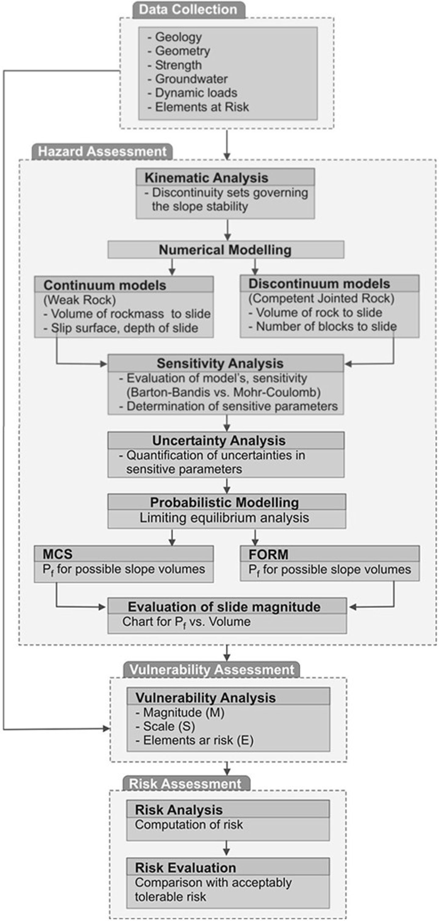
Figure 1 : Risk assessment framework for rock slopes
Hazard assessment
Hazards assessment is composed of the following consecutive stages:
Kinematic analysis: The basic aim of this stage is to determine discontinuity sets that govern the slope instability
Numerical modeling: This stage is for understanding the possible failure mechanism and better determination of failure surface and slope geometry. Continuum models are more appropriate for weak rock conditions, while discontinuum models are more suitable for competent rock situations. The outputs of this stage are the volume of the rock mass to slide, geometry of slip surface and depth of slide for weak rock and number of blocks to slide, and volume of sliding rock for competent rock.
Sensitivity analysis: This stage is for the evaluation of the model's sensitivity to input parameters. Here the sensitivity of Mohr-Coulomb and/or Barton-Bandis failure criteria which are the most frequently used failure criteria for rock slopes, can also be compared.
Uncertainty analysis: Before probabilistic modeling, uncertainty analysis is essential to obtain more realistic slope failure probabilities. The uncertainties associated with the most sensitive parameters are quantified and analyzed in this stage.
Probabilistic modeling: Failure probability for the rock slope can be evaluated based on Monte Carlo simulation (MCS) or First Order Reliability Method (FORM).
Evaluation of slide magnitude: The magnitude of the hazard can be assessed by constructing the probability of failure (Pf) versus possible rock block volumes.
Vulnerability assessment
In this case, the vulnerability assessment diminishes to 2-dimension as the scale is small. Then vulnerability can be assessed in a (n x m) matrix, where n is the type of elements at risk and m is the number of rock blocks to slide.
Risk assessment
Risk assessment starts with the computation of total and specific risks.
Case study 2: Slopes in clay
The zone assessed in this study is located in an urban area on the Southern coast of Norway, extending about 1 km along the banks of a river in the vicinity of a fjord.
The quaternary geology description indicates that the soils in the area are nor­mally consolidated. Typical soil profiles display a river sand layer at the surface with marine deposits down to bedrock. The transition from marine sediments to sand/gravel deposits is lower than the river water level, which means the clay deposits are exposed to river erosion. The sensitivity tests of the clay indicate "quick clay" behavior.

Figure 2 Model of the area under investigation
Hazard assessment To quantify hazard, a scenario-based second-moment probabilistic limit equilibrium approach is implemented. The slope stability analyses account for the spatial variability of undrained shear strength. Spatial variability of soil strength, river water level, and river bed erosion significantly influenced hazard and expected risk levels.
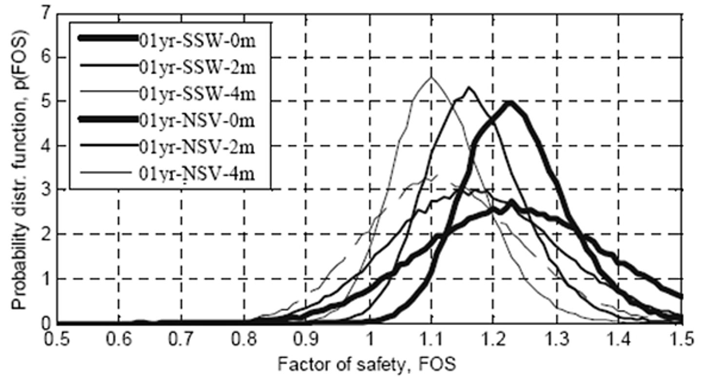
Figure 3 Probabaility distributions of calculated 3-D factor of safety for "01yr" scenarios
Vulnerability assessment Vulnerability and elements at risk are estimated with a second-moment approach. Values for vulnerability are obtained from published data and engineering judgment. Categories of elements at risk are considered in the study.
Risk assessment Risk estimates are based on hazard, vulnerability, and the potential loss associated with the elements at risk. The uncertainty in risk estimates is quantified using first-order second-moment approximation.
Case Study 3: Snow Avalanches
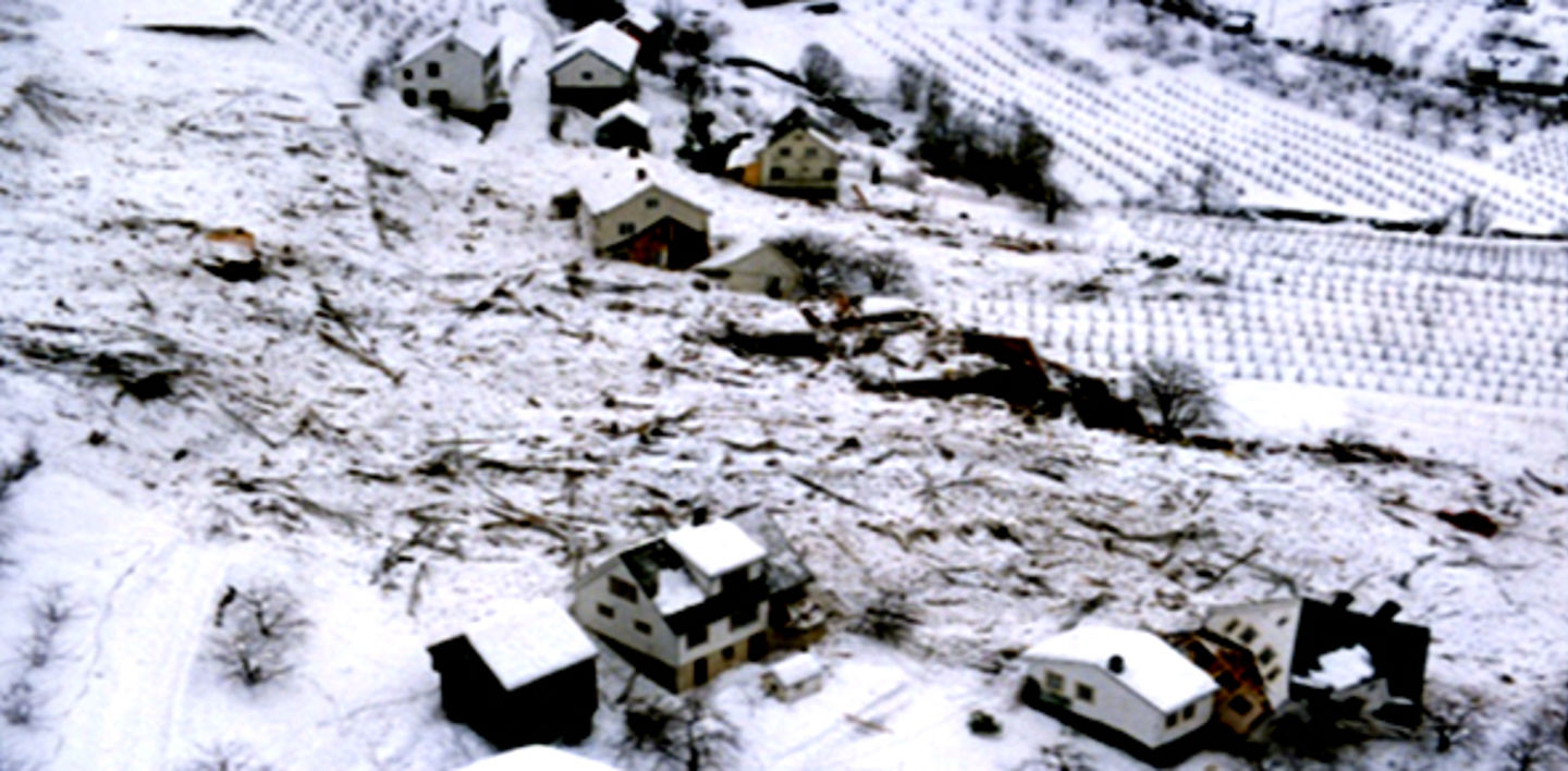
Figure 4 Snow avalange at Bleie, Norway
Avalanches constitute a considerable natural hazard in snow-covered mountain areas. They are fast-moving masses of snow and debris on (steep) mountain slopes, which can cause catastrophic destruction. During precipitation and/or storm periods, snow accumulates on slopes. Snow weight may exceed the shear resistance at some critical snow depth when the snow amount increases, and a slide will be released.
In addition, external loads can contribute to the release of a slab, like a skier, or loading by explosives as done for temporal mitigation. Also, reducing the strength, for example, due to rapid warming or rain, can cause an avalanche release. During their descent, avalanches may reach a velocity of up to 100 m/s; the flowing density is thought to range typically between 30 to 300 kg m3. Thus, impact pressures can be as high as several hundred kPa.
Two case studies for avalanches have been performed where hazard, vulnerability, and risk are estimated:
- a case regarding the risk to a building in an avalanche path*
- a study concerning the risk to traffic on a major mountain road
Here, the first of these case studies is presented.
- risk to a building in an avalanche path
- a farm is at the foot of an avalanche path at about 30 masl.
Hazard assessment
The hazard comprises two parts: the probability of release and the likelihood of run-out of a snow avalanche. Input parameters are:
meteorology parameter: precipitation
slide release parameters, see table below
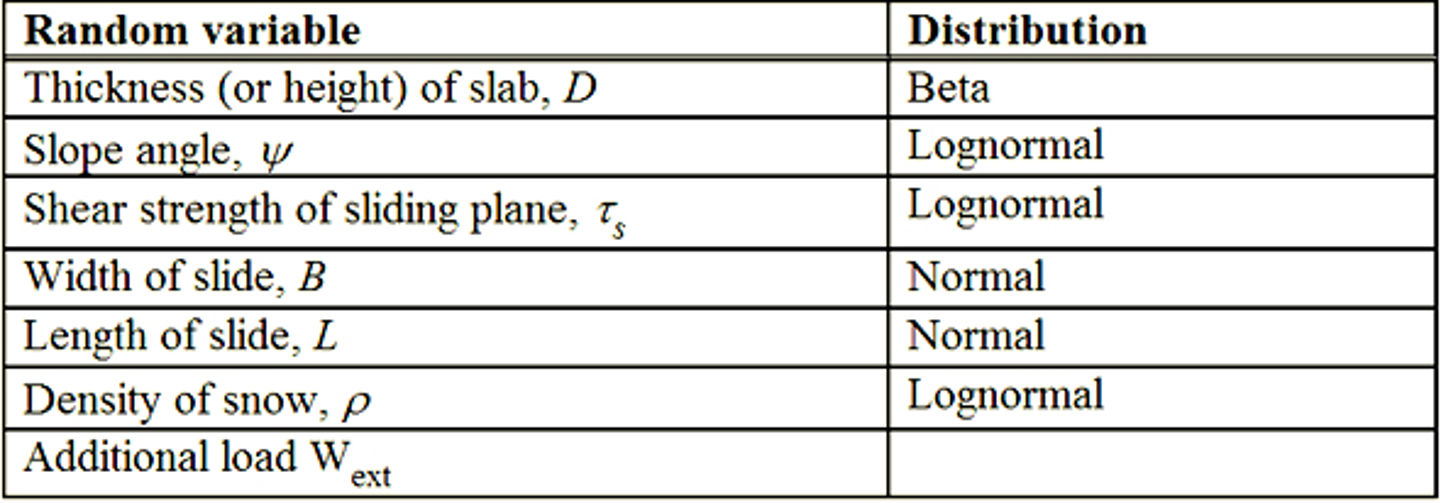
In the hazard assessment, the following models for release and run-out are used:
- Release model: A simple snow slab avalanche model predicts the release, see figure below. The release probability is denoted by P release. The probability of sliding, Pslide, is found by integrating Prelease's overall snow depths.
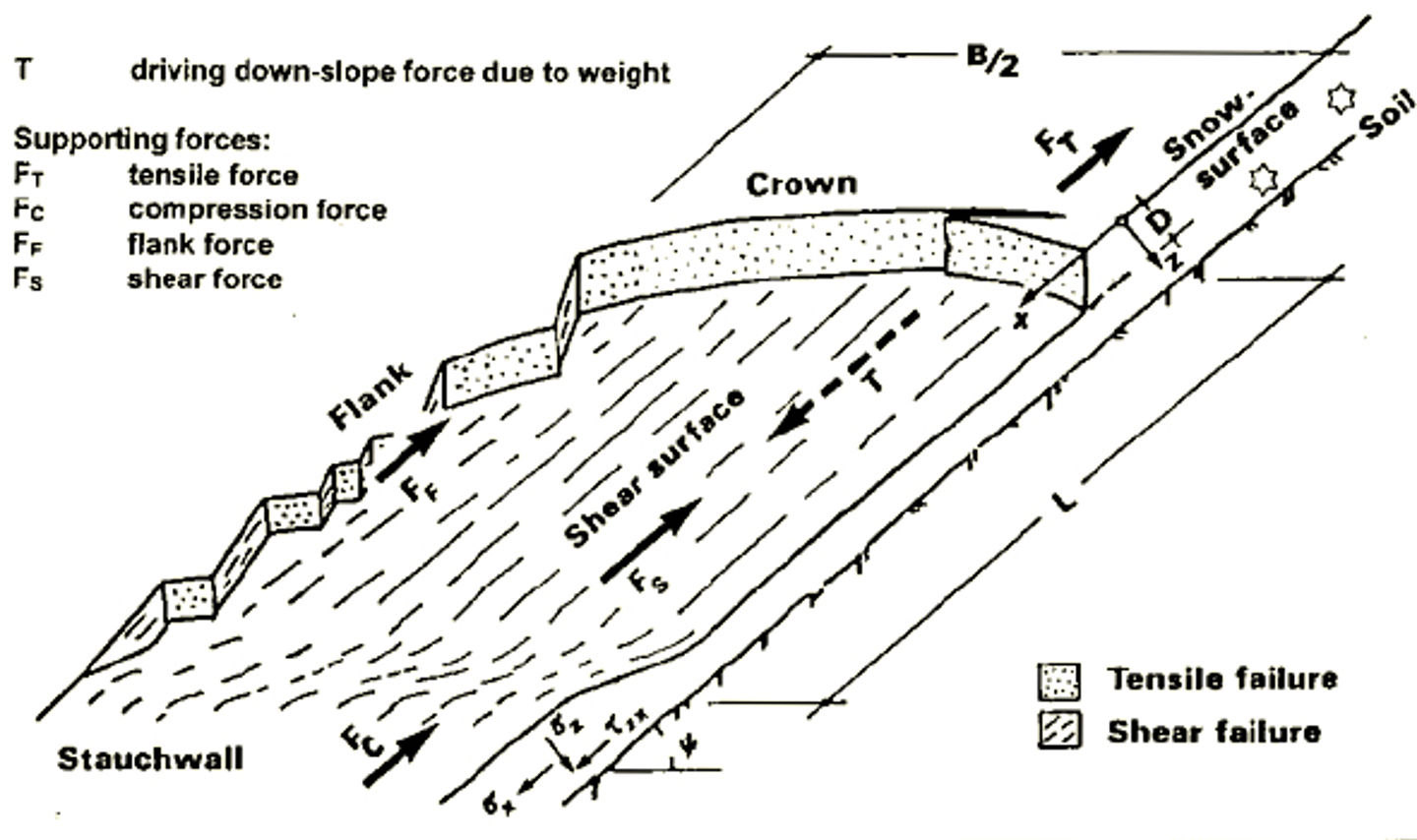
Figure 5 Snow-slab avalanche definitions, coordinate system and acting forces (Lackinger, 1989)
- Run-out model: An energy line approach combined with Monte Carlo simulation is used for run-out prediction. Based on simple energy considerations, the energy line approach allows us to determine the run-out length and to give an estimate of the velocity along the track:
Kinetic energy = loss of potential energy - energy loss due to friction
Ptravel denotes the run-out probability
The avalanche hazard at the farm location is given by the probability of the avalanche occurrence times the likelihood that the avalanche reaches the location:
H = Pslide- Ptravel
Vulnerability assessment
Vulnerability curves for both constant flow density and velocity-dependent density are given in the figure below.
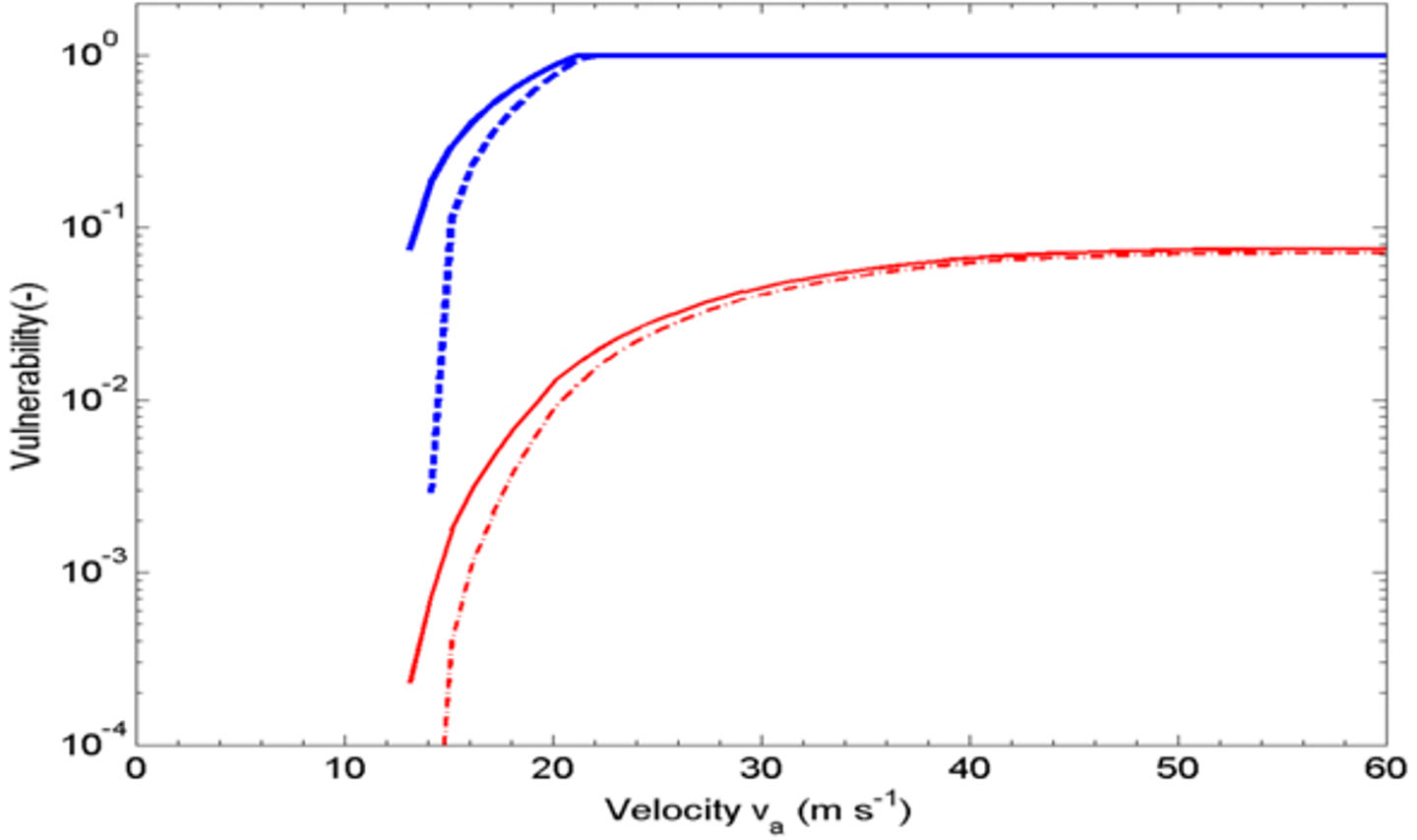
Figure 6 Cumulative vulnerability curve versus avalanche speed (red solid line velocity dependent density; red dashed line constant flow density). The blue lines show corresponding specific loss curve for a monumental buildings.
The vulnerability of a building is defined by integrating the probability of a specific loss over all speeds.
Risk assessment
- Building - the risk to a building is given by the product of hazard and the vulnerability of the specific building
- Inhabitants - the individual risk to a person is given by the product of hazard, vulnerability, and the exposure of the respective person
The risk estimation process is illustrated in the figure below.
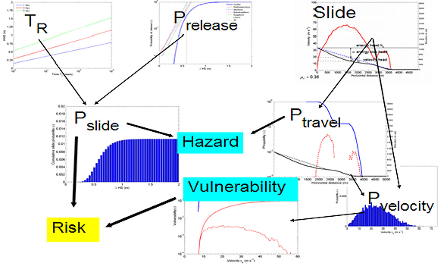
Figure 7 llustration of the steps in the risk assessment
Case Study 4: Tsunamis
The scope of the study is to quantify the risk associated with a rock slide at Åknes, which can potentially generate a tsunami. The Åknes rock slope is located in Storfjorden in Western Norway. The area has been subject to many rockslides during post-glacial time. In 1934 a rock slide hit the fjord near Tafjord, also in the Storfjorden area, and caused a disastrous tsunami that killed 41 people.
Data collection
Available literature has collected data about historical rockslides in the Storfjorden area. Data for the vulnerability has been collected from sources containing fatality rates from tsunamis in western Norway, from the December 2004 Indian Ocean tsunami, and from the July 2006 Java tsunami.
Hazard assessment
The Åknes threat is not the rockslide itself but its tsunamigenic potential. This means that the hazard is comprised of two parts:
- the probability of a rockslide at Åknes
- the likelihood of generating a tsunami caused by the Åknes rockslide
- the probability is calculated from the frequency of previous rockslides in the Storfjorden area and from expert judgment
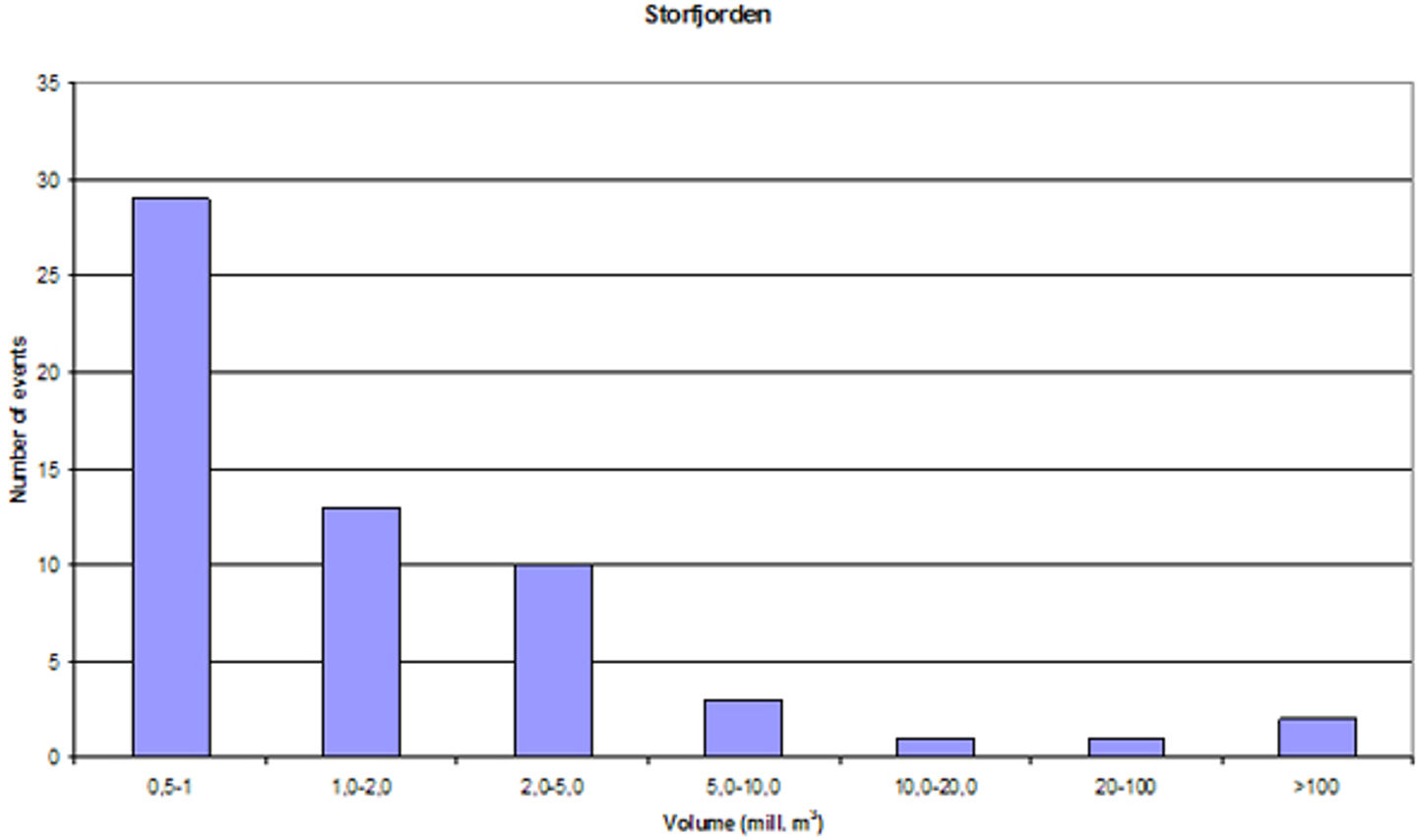
Figure 8 The diagram shows the number of rock-avalanche events and the volume distribution in the entire Storfjorden, Blikra et al. (2005).
The tsunami the rockslide generates is calculated by numerical simulation using linear shallow water equations. Several rock volumes are considered in the analysis. Corresponding run-up heights are computed for four different locations.
Vulnerability assessment
In this study, vulnerability to people is studied. The quantitative vulnerability models for people are based on historic data from statistics of previous tsunami disasters. This is obtained in two steps:
- a review of life's losses caused by earlier tsunamis
- a formulation of a continuous model relating inundation height with life's losses
Vulnerability curves are proposed for vulnerability as a function of inundation height, shown in the figure below.
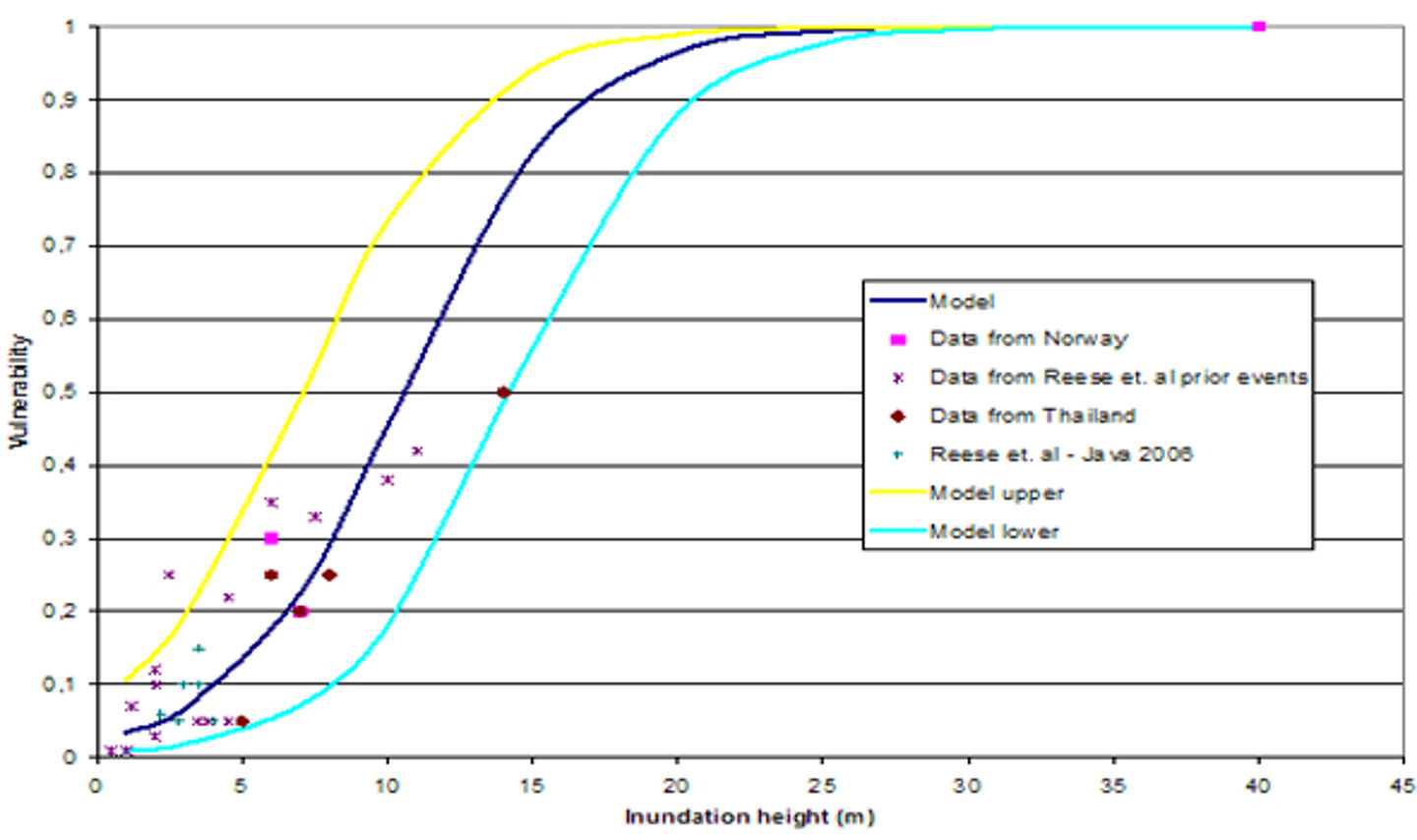
Figure 9 Empirical quantification of vulnerability as a function of inundation height
Risk assessment
Two approaches are proposed for quantifying risk at the prescribed locations in Storfjorden.
- an 'implicit' system I, based on the principle that the expected risk value equals the product of the predicted value of hazard, vulnerability, and losses, including an implicit relaxation on the dependencies between multi-threats
- the Bayesian network approach BN relates the causal dependencies between the threats and other relevant risk factors.